Low Latency Reads and Writes in a Multi-Region Cluster

CockroachDB multi-region capabilities make it easier to run global applications. For an overview of these capabilities, see . In multi-region clusters, the distribution of data becomes a performance consideration. This makes it important to think about the of each database. Then, for each table in the database, use the right to locate data for optimal performance. In this tutorial, you will:

Simulate a multi-region CockroachDB cluster on your local machine.
Run a workload on the cluster using our fictional vehicle-sharing application called .
See the effects of network latency on SQL query performance in the default (non-multi-region) configuration.
Configure the cluster for good multi-region performance by issuing SQL statements that choose the right and .

Considerations

This page describes a demo cluster; it does not show best practices for a production deployment. For more information about production deployments of multi-region applications, see and the . Because the instructions on this page describe how to simulate a multi-region cluster on a single machine, the absolute performance numbers described below are not reflective of . Instead, the instructions are designed with the following goals:

To show the relative magnitude of the performance improvements to expect when you configure a multi-region cluster correctly.
To be as easy to try as possible with minimal configuration and setup.

Before you begin

Make sure you have:

A basic understanding of the MovR application
Docker installed on the local machine

A basic understanding of the MovR application

The workload you’ll run against the cluster is our open-source, fictional, peer-to-peer vehicle-sharing app, . Each instance represents users in a specific region:

europe-west1, covering the cities of Amsterdam, Paris, and Rome.
us-east1, covering the cities of New York, Boston, and Washington, D.C.
us-west1, covering the cities of Los Angeles, San Francisco, and Seattle.

The MovR schema

The six tables in the movr database store user, vehicle, and ride data for MovR:

Table	Description
`users`	People registered for the service.
`vehicles`	The pool of vehicles available for the service.
`rides`	When and where users have rented a vehicle.
`promo\_codes`	Promotional codes for users.
`user\_promo\_codes`	Promotional codes in use by users.
`vehicle\_location\_histories`	Vehicle location history.

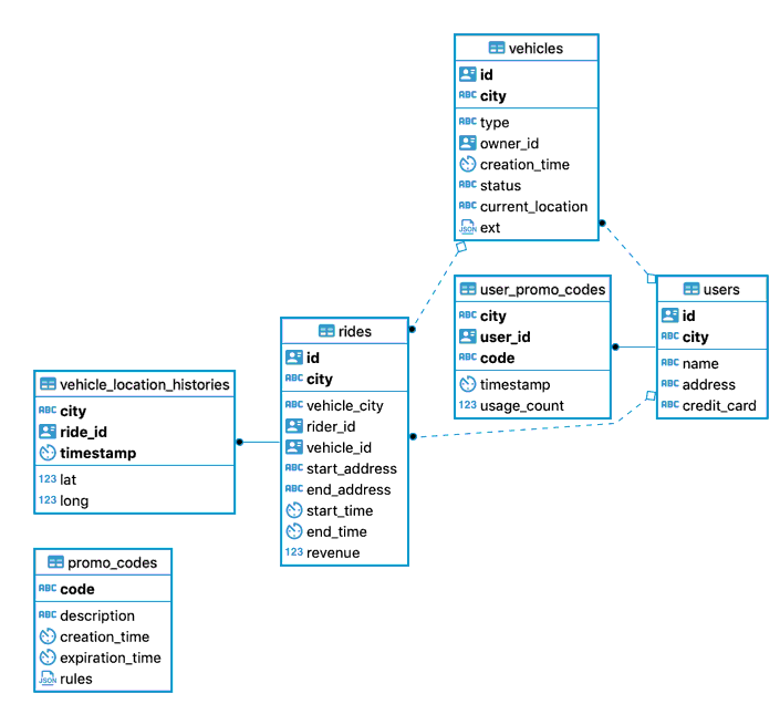
All of the tables except promo_codes have a composite primary key of city and id, in that order. This means that the rows in these tables are ordered by their geography. These tables are read from and written to very frequently. To keep read and write latency low, you’ll use the for these tables. The data in the promo_codes table is different: it is not tied to geography, and it is rarely updated. This type of table is often referred to as a “reference table” or “lookup table”. In this case, you’ll use the to keep read latencies low. For a description of the sequence of SQL statements issued by the MovR application in response to user actions, see .

Step 1. Simulate a multi-region cluster

Use the following command to start the cluster. This particular combination of flags results in a demo cluster of 9 nodes, with 3 nodes in each region. It sets the appropriate and also simulates the network latency that would occur between nodes in these localities. For more information about each flag, see the documentation, especially for .

$ cockroach demo --global --nodes 9 --no-example-database --insecure

When the cluster starts, you’ll see a message like the one shown below, followed by a SQL prompt. Note the URLs for:

Viewing the : http://127.0.0.1:8080.
Connecting to the database from a or a : postgres://root@127.0.0.1:26257?sslmode=disable.

#
# Welcome to the CockroachDB demo database!
#
# You are connected to a temporary, in-memory CockroachDB cluster of 9 nodes.
#
# This demo session will attempt to enable enterprise features
# by acquiring a temporary license from Cockroach Labs in the background.
# To disable this behavior, set the environment variable
# COCKROACH_SKIP_ENABLING_DIAGNOSTIC_REPORTING=true.
#
# Reminder: your changes to data stored in the demo session will not be saved!
#
# Connection parameters:
#   (webui)    http://127.0.0.1:8080/demologin?password=demo76950&username=demo
#   (sql)      postgres://demo:demo76950@127.0.0.1:26257?sslmode=require
#   (sql/unix) postgres://demo:demo76950@?host=%2Fvar%2Ffolders%2Fc8%2Fb_q93vjj0ybfz0fz0z8vy9zc0000gp%2FT%2Fdemo070856957&port=26257
#
# To display connection parameters for other nodes, use \demo ls.
#
# The user "demo" with password "demo76950" has been created. Use it to access the Web UI!
#
# Server version: CockroachDB CCL v21.1.2 (x86_64-apple-darwin19, built 2021/06/07 18:13:04, go1.15.11) (same version as client)
# Cluster ID: bfd9fc91-69bd-4417-a2f7-66e556bf2cfd
# Organization: Cockroach Demo
#
# Enter \? for a brief introduction.
#

To verify that the simulated latencies are working as expected, check the in the DB Console. Round trip times between us-west1 and europe-west1 should be in the 150 ms range.

Step 2. Determine node locations

To determine which nodes are in which regions, you will need to refer to two (2) things:

The output of the \demo ls from the SQL shell, which shows the TCP ports on the local machine that we will connect to from the MovR application.
The node IDs shown on the Network Latency Page.

Here is the output of \demo ls from the SQL shell.

> \demo ls

node 1:
  (webui)    http://127.0.0.1:8080/demologin?password=demo76950&username=demo
  (sql)      postgres://demo:demo76950@127.0.0.1:26257?sslmode=require
  (sql/unix) postgres://demo:demo76950@?host=%2Fvar%2Ffolders%2Fc8%2Fb_q93vjj0ybfz0fz0z8vy9zc0000gp%2FT%2Fdemo070856957&port=26257

node 2:
  (webui)    http://127.0.0.1:8081/demologin?password=demo76950&username=demo
  (sql)      postgres://demo:demo76950@127.0.0.1:26258?sslmode=require
  (sql/unix) postgres://demo:demo76950@?host=%2Fvar%2Ffolders%2Fc8%2Fb_q93vjj0ybfz0fz0z8vy9zc0000gp%2FT%2Fdemo070856957&port=26258

node 3:
  (webui)    http://127.0.0.1:8082/demologin?password=demo76950&username=demo
  (sql)      postgres://demo:demo76950@127.0.0.1:26259?sslmode=require
  (sql/unix) postgres://demo:demo76950@?host=%2Fvar%2Ffolders%2Fc8%2Fb_q93vjj0ybfz0fz0z8vy9zc0000gp%2FT%2Fdemo070856957&port=26259

node 4:
  (webui)    http://127.0.0.1:8083/demologin?password=demo76950&username=demo
  (sql)      postgres://demo:demo76950@127.0.0.1:26260?sslmode=require
  (sql/unix) postgres://demo:demo76950@?host=%2Fvar%2Ffolders%2Fc8%2Fb_q93vjj0ybfz0fz0z8vy9zc0000gp%2FT%2Fdemo070856957&port=26260

node 5:
  (webui)    http://127.0.0.1:8084/demologin?password=demo76950&username=demo
  (sql)      postgres://demo:demo76950@127.0.0.1:26261?sslmode=require
  (sql/unix) postgres://demo:demo76950@?host=%2Fvar%2Ffolders%2Fc8%2Fb_q93vjj0ybfz0fz0z8vy9zc0000gp%2FT%2Fdemo070856957&port=26261

node 6:
  (webui)    http://127.0.0.1:8085/demologin?password=demo76950&username=demo
  (sql)      postgres://demo:demo76950@127.0.0.1:26262?sslmode=require
  (sql/unix) postgres://demo:demo76950@?host=%2Fvar%2Ffolders%2Fc8%2Fb_q93vjj0ybfz0fz0z8vy9zc0000gp%2FT%2Fdemo070856957&port=26262

node 7:
  (webui)    http://127.0.0.1:8086/demologin?password=demo76950&username=demo
  (sql)      postgres://demo:demo76950@127.0.0.1:26263?sslmode=require
  (sql/unix) postgres://demo:demo76950@?host=%2Fvar%2Ffolders%2Fc8%2Fb_q93vjj0ybfz0fz0z8vy9zc0000gp%2FT%2Fdemo070856957&port=26263

node 8:
  (webui)    http://127.0.0.1:8087/demologin?password=demo76950&username=demo
  (sql)      postgres://demo:demo76950@127.0.0.1:26264?sslmode=require
  (sql/unix) postgres://demo:demo76950@?host=%2Fvar%2Ffolders%2Fc8%2Fb_q93vjj0ybfz0fz0z8vy9zc0000gp%2FT%2Fdemo070856957&port=26264

node 9:
  (webui)    http://127.0.0.1:8088/demologin?password=demo76950&username=demo
  (sql)      postgres://demo:demo76950@127.0.0.1:26265?sslmode=require
  (sql/unix) postgres://demo:demo76950@?host=%2Fvar%2Ffolders%2Fc8%2Fb_q93vjj0ybfz0fz0z8vy9zc0000gp%2FT%2Fdemo070856957&port=26265

And here is the view on the Network Latency Page, which shows which nodes are in which cluster regions:

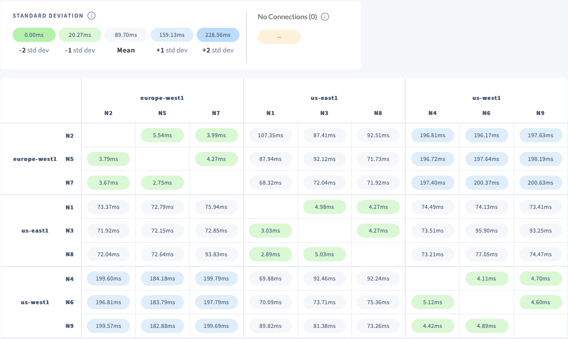
You can see by referring back and forth between \demo ls and the Network Latency Page that the cluster has the following region/node/port correspondences, which we can use to determine how to connect MovR from various regions:

Node ID	Region	Port on localhost
N2	europe-west1	26263
N5	europe-west1	26264
N7	europe-west1	26265
N4	us-west1	26262
N6	us-west1	26260
N9	us-west1	26261
N1	us-east1	26257
N3	us-east1	26259
N8	us-east1	26258

Step 3. Load and run MovR

Follow these steps to start 3 instances of MovR. Each instance is pointed at a node in a different region. This will simulate load from that region.

In the SQL shell, create the movr database:
CREATE DATABASE IF NOT EXISTS movr;

Open a second terminal and run the command below to populate the MovR data set. The options are mostly self-explanatory. We limit the application to 1 thread because using multiple threads quickly overloads this small demo cluster’s ability to ingest data. As a result, loading the data takes about 90 seconds on a fast laptop.

    docker run -it --rm cockroachdb/movr:20.11.1 \
        --app-name "movr-load" \
        --url "postgres://root@docker.for.mac.localhost:26257/movr?sslmode=disable" \
        --num-threads 1 \
        load \
        --num-users 100 \
        --num-rides 100 \
        --num-vehicles 10 \
        --city "boston" \
        --city "new york" \
        --city "washington dc" \
        --city="amsterdam" \
        --city="paris" \
        --city="rome" \
        --city="los angeles" \
        --city="san francisco" \
        --city="seattle"

[INFO] (MainThread) connected to movr database @ postgres://root@docker.for.mac.localhost:26257/movr?sslmode=disable
[INFO] (MainThread) Loading single region MovR
[INFO] (MainThread) initializing tables
[INFO] (MainThread) loading cities ['boston', 'new york', 'washington dc', 'amsterdam', 'paris', 'rome', 'los angeles', 'san francisco', 'seattle']
[INFO] (MainThread) loading movr data with ~100 users, ~10 vehicles, ~100 rides, ~1000 histories, and ~1000 promo codes
[INFO] (Thread-1  ) Generating user data for boston...
... output snipped ...
[INFO] (Thread-1  ) Generating 1000 promo codes...
[INFO] (MainThread) populated 9 cities in 86.986230 seconds

In the same terminal window, run the following command:

docker run -it --rm cockroachdb/movr:20.11.1 \
    --app-name "movr-us-east" \
    --url "postgres://root@docker.for.mac.localhost:26257/movr?sslmode=disable" \
    run \
    --city="boston" \
    --city="new york" \
    --city="washington dc"

[INFO] (MainThread) connected to movr database @ postgres://root@docker.for.mac.localhost:26257/movr?sslmode=disable
[INFO] (MainThread) simulating movr load for cities ['boston', 'new york', 'washington dc']
[INFO] (MainThread) warming up....
[INFO] (MainThread) running single region queries...
...

Open a third terminal and run the following command:

docker run -it --rm cockroachdb/movr:20.11.1 \
    --app-name "movr-us-west" \
    --url "postgres://root@docker.for.mac.localhost:26260/movr?sslmode=disable" \
    run \
    --city="los angeles" \
    --city="san francisco" \
    --city="seattle"

[INFO] (MainThread) connected to movr database @ postgres://root@docker.for.mac.localhost:26260/movr?sslmode=disable
[INFO] (MainThread) simulating movr load for cities ['los angeles', 'san francisco', 'seattle']
[INFO] (MainThread) warming up....
[INFO] (MainThread) running single region queries...

Open a fourth terminal and run the following command:

docker run -it --rm cockroachdb/movr:20.11.1 \
   --app-name "movr-eu-west" \
   --url "postgres://root@docker.for.mac.localhost:26264/movr?sslmode=disable" \
   run \
   --city="amsterdam" \
   --city="paris" \
   --city="rome"

[INFO] (MainThread) connected to movr database @ postgres://root@docker.for.mac.localhost:26264/movr?sslmode=disable
[INFO] (MainThread) simulating movr load for cities ['amsterdam', 'paris', 'rome']
[INFO] (MainThread) warming up....
[INFO] (MainThread) running single region queries...
...

Step 4. Check service latency

Now that you have load hitting the cluster from different regions, check how the service latencies look before you do any multi-region configuration from SQL. This is the “before” case in the “before and after”. In the at http://127.0.0.1:8080, click on the left and hover over the timeseries graph. You should see the effects of network latency on this workload.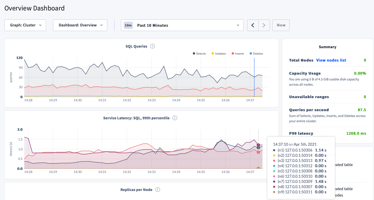

For each of the 3 nodes that you are pointing the movr workload at, the max latency of 99% of queries are in the 1-2 seconds range. The SQL latency is high because of the network latency between regions. To see the network latency between any two nodes in the cluster, click in the left-hand navigation.

Within a single region, round-trip latency is under 6 ms (milliseconds). Across regions, round-trip latency is significantly higher. For example:

Round-trip latency between N2 in europe-west1 and N3 in us-east1 is 87 ms.
Round-trip latency between N2 in europe-west1 and N4 in us-west1 is 196 ms.

Step 5. Execute multi-region SQL statements

The following SQL statements will configure:

The database’s available regions.
Which data should be optimized for access from which region.

This information is necessary so that CockroachDB can move data around to optimize access to particular data from particular regions. The main focus is reducing latency in a global deployment. For more information about how this works at a high level, see the .

The following ALTER statements will take some seconds to run, since the cluster is under load.

Configure database regions

Back in the SQL shell, switch to the movr database:

USE movr;

Execute the following statements. They will tell CockroachDB about the database’s regions. This information is necessary so that CockroachDB can later move data around to optimize access to particular data from particular regions. For more information about how this works at a high level, see .

ALTER DATABASE movr PRIMARY REGION "us-east1";
ALTER DATABASE movr ADD REGION "europe-west1";
ALTER DATABASE movr ADD REGION "us-west1";

Configure table localities

Configure GLOBAL tables

As mentioned earlier, all of the tables except promo_codes are geographically specific. Because the data in promo_codes is not updated frequently (a.k.a., “read-mostly”), and needs to be available from any region, the right table locality is .

ALTER TABLE promo_codes SET locality GLOBAL;

Next, alter the user_promo_codes table to have a foreign key into the global promo_codes table. This will enable fast reads of the promo_codes.code column from any region in the cluster.

ALTER TABLE user_promo_codes
  ADD CONSTRAINT user_promo_codes_code_fk
    FOREIGN KEY (code)
    REFERENCES promo_codes (code)
    ON UPDATE CASCADE;

Configure REGIONAL BY ROW tables

All of the tables except promo_codes contain rows which are partitioned by region, and updated very frequently. For these tables, the right table locality for optimizing access to their data is . Apply this table locality to the remaining tables. These statements use a CASE statement to put data for a given city in the right region and can take around 1 minute to complete for each table.

rides

ALTER TABLE rides ADD COLUMN region crdb_internal_region AS (
  CASE WHEN city = 'amsterdam' THEN 'europe-west1'
       WHEN city = 'paris' THEN 'europe-west1'
       WHEN city = 'rome' THEN 'europe-west1'
       WHEN city = 'new york' THEN 'us-east1'
       WHEN city = 'boston' THEN 'us-east1'
       WHEN city = 'washington dc' THEN 'us-east1'
       WHEN city = 'san francisco' THEN 'us-west1'
       WHEN city = 'seattle' THEN 'us-west1'
       WHEN city = 'los angeles' THEN 'us-west1'
  END
) STORED;
ALTER TABLE rides ALTER COLUMN REGION SET NOT NULL;
ALTER TABLE rides SET LOCALITY REGIONAL BY ROW AS "region";

user_promo_codes

ALTER TABLE user_promo_codes ADD COLUMN region crdb_internal_region AS (
  CASE WHEN city = 'amsterdam' THEN 'europe-west1'
       WHEN city = 'paris' THEN 'europe-west1'
       WHEN city = 'rome' THEN 'europe-west1'
       WHEN city = 'new york' THEN 'us-east1'
       WHEN city = 'boston' THEN 'us-east1'
       WHEN city = 'washington dc' THEN 'us-east1'
       WHEN city = 'san francisco' THEN 'us-west1'
       WHEN city = 'seattle' THEN 'us-west1'
       WHEN city = 'los angeles' THEN 'us-west1'
  END
) STORED;
ALTER TABLE user_promo_codes ALTER COLUMN REGION SET NOT NULL;
ALTER TABLE user_promo_codes SET LOCALITY REGIONAL BY ROW AS "region";

users

ALTER TABLE users ADD COLUMN region crdb_internal_region AS (
  CASE WHEN city = 'amsterdam' THEN 'europe-west1'
       WHEN city = 'paris' THEN 'europe-west1'
       WHEN city = 'rome' THEN 'europe-west1'
       WHEN city = 'new york' THEN 'us-east1'
       WHEN city = 'boston' THEN 'us-east1'
       WHEN city = 'washington dc' THEN 'us-east1'
       WHEN city = 'san francisco' THEN 'us-west1'
       WHEN city = 'seattle' THEN 'us-west1'
       WHEN city = 'los angeles' THEN 'us-west1'
  END
) STORED;
ALTER TABLE users ALTER COLUMN REGION SET NOT NULL;
ALTER TABLE users SET LOCALITY REGIONAL BY ROW AS "region";

vehicle_location_histories

ALTER TABLE vehicle_location_histories ADD COLUMN region crdb_internal_region AS (
  CASE WHEN city = 'amsterdam' THEN 'europe-west1'
       WHEN city = 'paris' THEN 'europe-west1'
       WHEN city = 'rome' THEN 'europe-west1'
       WHEN city = 'new york' THEN 'us-east1'
       WHEN city = 'boston' THEN 'us-east1'
       WHEN city = 'washington dc' THEN 'us-east1'
       WHEN city = 'san francisco' THEN 'us-west1'
       WHEN city = 'seattle' THEN 'us-west1'
       WHEN city = 'los angeles' THEN 'us-west1'
  END
) STORED;
ALTER TABLE vehicle_location_histories ALTER COLUMN REGION SET NOT NULL;
ALTER TABLE vehicle_location_histories SET LOCALITY REGIONAL BY ROW AS "region";

vehicles

ALTER TABLE vehicles ADD COLUMN region crdb_internal_region AS (
  CASE WHEN city = 'amsterdam' THEN 'europe-west1'
       WHEN city = 'paris' THEN 'europe-west1'
       WHEN city = 'rome' THEN 'europe-west1'
       WHEN city = 'new york' THEN 'us-east1'
       WHEN city = 'boston' THEN 'us-east1'
       WHEN city = 'washington dc' THEN 'us-east1'
       WHEN city = 'san francisco' THEN 'us-west1'
       WHEN city = 'seattle' THEN 'us-west1'
       WHEN city = 'los angeles' THEN 'us-west1'
  END
) STORED;
ALTER TABLE vehicles ALTER COLUMN REGION SET NOT NULL;
ALTER TABLE vehicles SET LOCALITY REGIONAL BY ROW AS "region";

Step 6. Re-check service latency

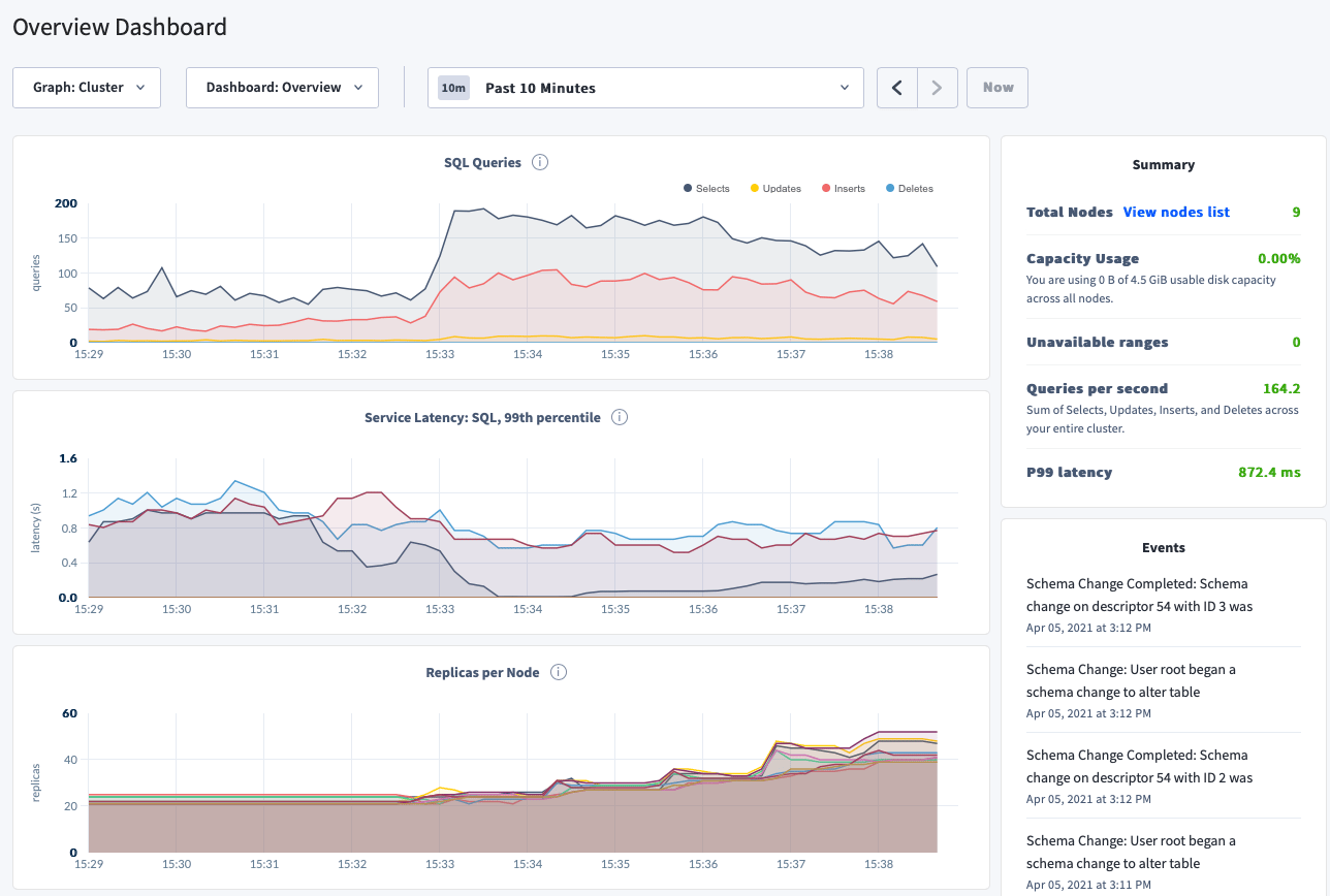
As the multi-region schema changes complete, you should see changes to the following metrics:

SQL Queries: This number should go up, since the cluster can service more load due to better performance (due to better data locality and lower latency). In this particular run, the QPS has almost doubled, from 87 to 164.
Service Latency: SQL, 99th percentile: In general, even on a small demo cluster like this, the P99 latency should drop and also get less spiky over time, as schema changes finish and data is moved around. For this particular run, the P99 latency has dropped from ~1200 ms to ~870 ms, an over 25% improvement.
Replicas per Node: This will increase, since the data needs to be spread across more nodes in order to service the multi-region workload appropriately. There is nothing you need to do about this, except to note that it happens, and is required for CockroachDB’s improved multi-region performance features to work.

The small demo cluster used in this example is essentially in a state of overload from the start. The performance numbers shown here only reflect the direction of the performance improvements. You should expect to see much better absolute performance numbers than those described here .

​Considerations

​Before you begin

​A basic understanding of the MovR application

​The MovR schema

​Step 1. Simulate a multi-region cluster

​Step 2. Determine node locations

​Step 3. Load and run MovR

​Step 4. Check service latency

​Step 5. Execute multi-region SQL statements

​Configure database regions

​Configure table localities

​Configure GLOBAL tables

​Configure REGIONAL BY ROW tables

​Step 6. Re-check service latency

​See also

Considerations

Before you begin

A basic understanding of the MovR application

The MovR schema

Step 1. Simulate a multi-region cluster

Step 2. Determine node locations

Step 3. Load and run MovR

Step 4. Check service latency

Step 5. Execute multi-region SQL statements

Configure database regions

Configure table localities

Configure GLOBAL tables

Configure REGIONAL BY ROW tables

Step 6. Re-check service latency

See also